- Intro
- The Forward Process
- The Score Function
- Learning the Score Function
- The Reverse Process
- Conditional Generation and Classifier-Free Guidance
- Implementation Details
Note that equations that overflow horizontally are scrollable!
Intro
I had heard of diffusion models numerous times in the context of generative AI for image generation, but had never really taken interest in how they worked. A few months ago, I was lucky enough to stumble upon Peter Holderrieth and Ezra Erives' wonderful lectures. This is an incredible introductory resource on the topic, and the accompanying lecture notes and labs are extremely well put together. The first thing that came to mind when I started learning about diffusion was implementing one of these models from scratch in PyTorch. The lectures and other sources I've stumbled upon introduce some math ideas that I thought were interesting, so I had the idea of writing these notes detailing all I've learned. In particular, I hope to write it in a structured manner such that I can use this as a resource for future reference, and it may serve other people. Feel free to shoot me a message with any suggestions, corrections or critiques (contact information on this webpage).
When researching about generative models (for images in particular), you'll probably hear about Generative Adversarial Networks (GANs). I won't get too into it, but the neat part about GANs is that they consist two models: a Generator network, which is responsible for generating new samples, and a Discriminator network, that is trained to be able to tell if a sample is from the generator (fake) or from the actual dataset (real). This style of adversarial training has its advantages, interestingly, I've seen it used for neural-network based audio compression (See [1]). However, from my understanding, these have largely been replaced by Diffusion models nowadays (e.g StableDiffusion 3, Dall-E, Sora). GANs suffer from issues like training instability (due to this dual model approach) and mode collapse (output becomes limited to a subset of the actual distribution). Whereas with diffusion, common training objectives are quite simple, consisting of using some kind of Neural Network (NN) to learn to predict the noise, or to give us a score. Diffusion also offers a very clear mathematical framework for generating/sampling from our dataset's distribution.
I'll be assuming a certain level of math background, but the main concepts will be explained as they come up. I'll assume familiarity with: vectors, matrices, PDFs, gaussian distributions, calculus, differential equations, and obviously principles of deep learning. Also, keep in mind there are a few different variations of diffusion denoisers (different learning objective, discrete vs continuous definitions). My implementation uses a continuous-time score-matching approach, and some definitions and equations from [2]. This one is interesting specifically because it uses the differential equations we'll see here to build a sort of framework for different types of diffusion.
Here is the github repo with my implementation: https://github.com/joaovdonaton/diffusion-zero
The Forward Process
Now, onto the actual model. Our goal is to create something that can generate coherent images that are similar to the ones in our training dataset. We'll assume there exists a probability distribution that describes our train set: $P_{data}$. We represent each of our images' pixel values as a really high dimensional vector $x \in \mathbb{R}^d$, where $x_0 \sim P_{data}$. However, a central issue here is that in practice we cannot sample from $P_{data}$. All we have are a limited number of samples from it. The whole idea behind diffusion denoising is, we start at noise sampled from something like $\mathcal{N}(0, I_d)$ (standard gaussian) and somehow move towards a sample that is around the high density areas of our $P_{data}$, which should consist of coherent images. We do this by defining a forward noising process, that takes an actual image from our train set, and gradually noises it, until we end up with complete noise (in a distribution that we can get the probability density for). Then, it's possible (though not simple) to derive a reverse process, that takes us from this noise, to a sample.
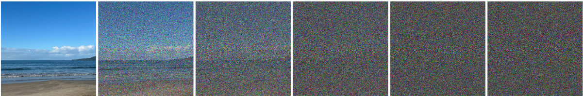
Forward process in 6 discrete timesteps.
The forward process can be expressed in terms of a Stochastic Differential Equation (SDE):
$$dx = f(x, t)dt + g(t)dW$$Let's look at this in parts. The $dx$ term just tells us this represents a small change in $x$ (remember $x$ starts at an actual image here). This equation tells us how to update $dx$. $dt$ is a small change in time, this change from sample to noise and the reverse is modelled as a function of time, I'll use $t=0$ as the initial time of a clean sample, and $t=1$ as the final time, where we have a noised sample. What's interesting here is the $dW$ term, this is what makes this equation Stochastic. It is defined as:
$$dW \sim \mathcal{N}(0, I_ddt)$$This is actually called Brownian Motion. In short, random noise pulled from a Gaussian Distribution centered at 0, and scaled by the change in time. And it describes how noise is added to $x$ at each timestep. Fun fact, in physics, brownian motion describes the randomness of the movements of particles suspended under certain conditions. An important property that should be clear is that the changes from $t$ to $t+1$ are completely independent of whatever happened before (aka the Markov property).
We also have $f(x, t)$, the drift coefficient and $g(t)$ the diffusion coefficient. These are strategically defined to be functions such that we end up at our desired distribution at the end of the forward process. There are two common variations of this, the Variance Exploding (VE) and Variance Preserving (VP) processes. My first attempt at implementing this was actually using VE, but I had trouble getting it to work, so I switched to VP. One thing you'll notice with the implementation of these equations is that it's pretty easy to run into numerical issues (zero division, explosion). For the purposes of this implementation, we'll focus on VP, which is set up in a way that we always end up with $x_1 \sim \mathcal{N}(0,I_d)$ (notice the notation, $x_1$ is sample at $t=1$, i.e after forward process). Here's the VP forward:
$$dx_t = -\frac{1}{2}\beta (t) x_t dt + \sqrt{\beta (t)}dW$$Where we pick:
$$\beta (t) = \beta_{min} + t(\beta_{max} - \beta_{min})$$This is called a Noise Schedule, here $\beta(t)$ linearly moves from $\beta_{min}$ to $\beta_{max}$ (I use 0.1 and 20 respectively, same as in [2]). To actually implement the forward process (we use it during training, we'll get there in a bit), we need to discretize it. We want to be able to pick a $t \in [0,1]$, and get a version of the sample $x_t$ with the appropriate amount of noise for that point in the noising. We do this by using an $\bar{\alpha}(t) = exp(-\int_0^t{\beta(t)}dt)$, which in short tells us how much of the original image is retained at time $t$. Basically, for $\beta(t)$ as $t \rightarrow 1$, we'll get a larger accumulation of noise, and have a smaller amount of the actual image remaining. Skipping the derivation, it turns out that the forward SDE has a solution for this:
Which we can easily implement in PyTorch to get samples $x_t$ at any $t$ stage of noising. If, like me, you were wondering why this preserves variance to $1$. It's pretty simple to show: our data samples are normalized using $\frac{x-mean}{std}$, which means over our dataset each sample has unit variance. And obviously $Var(\epsilon)=1$. So if we want the variance of $x_t$, we can use the fact that both $x_0$ and $\epsilon$ are independent, and use the linearity and properties of variance to get:
Great! now we have a concrete way of defining how we move from a sample from our dataset ($x_0$) to a sample that consists of noise pulled from a standard gaussian distribution ($x_1$). Next, we'll use these to define our reverse process and score, and elaborate on how training and inference makes use of these.
The Score Function
Before getting to the reverse process, we must understand what "score" refers to here (this is diffusion via score matching after all). For probability density function $p_t$ ($p$ is different at every $t$ because of the forward process, we have a slightly different distribution at different $t$'s), our conditional score is defined as:
$$\nabla_x \, log \;p_t(x|x_0) $$We can read this as "gradient of the $log$ likelihood of $x$ given $x_0$". Remember that $x_0$ is from our dataset $P_{data}$, so here our score is called conditional because $p_t(x|x_0)$ gives us the density (i.e how concentrated) of $x$ assuming that we are starting from $x_0$. This function is useful because the gradient gives us the direction of greatest ascent at a point $x$, so if we take our $x+\nabla_x \, log \;p_t(x|x_0) $, we are essentially moving in the direction of higher density regions of our distribution. Due to our forward process, this higher density region corresponds to a slightly less noisy version of $x$ (because it's a gaussian centered at factor of $x_0$). This works similarly to gradient descent, in the sense that we can start at a point, and gradually move according to the gradient until we end up close to an extreme.
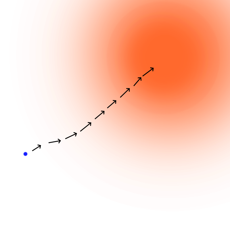
2D visualization of moving in the direction of the score. The blue dot would be our $x_t$. The orange region corresponds to a high density area for a given $p_t$
Now, it turns out that for our conditional score, it's not hard to derive an easily computable form for it. And I think it's kind of cool, so I will show the derivation. Remember we are using $x_t = x_0\sqrt{\bar{\alpha}(t)}+ \epsilon\sqrt{1 - \bar{\alpha}(t)}, \,\,\, \epsilon \in \mathcal{N}(0, I_d)$ from before as our $x_t$ in the forward, this has mean $\mu = x_0\sqrt{\bar{\alpha}(t)}$ and variance $\sigma^2 = 1-\bar{\alpha}(t)$ (note that variance here is different, because we are only considering a single fixed $x_0$, which will not have variance, whereas before we were looking at variance of $x_0$ over all samples). So, we have $p_t=\mathcal{N}(x_0\sqrt{\bar{\alpha}(t)}, (1-\bar{\alpha}(t))I_d)$ is a gaussian. Since this is the case, we actually have an expressin for a conditional $p_t$, using the d-dimensional isotropic gaussian equation! (see end of [3]):
With this, we can take the log:
Then take the gradient w.r.t $x$ and plug in our $\mu$ and $\sigma^2$:
We can rewrite our $x_t = x_0\sqrt{\bar{\alpha}(t)}+ \epsilon\sqrt{1 - \bar{\alpha}(t)}$, to show that the numerator from above is actually ${x_t-x_0\sqrt{\bar{\alpha}(t)}}=\epsilon {\sqrt{1 - \bar{\alpha}(t)}}$, plug in and we finally get:
What we have just derived is the exact expression we'll use in our loss function. We'll get to the algorithm and loss definition. But for now, we understand the what and the why of the score function. This expression is also interesting because it tells us that the score can be written in terms of the noise $\epsilon$ in this case. In fact, it's not hard to adapt this to train a noise predictor network (used in the paper that popularized diffusion models for image generation, [4]), instead of the score network. So, to recap, we can now compute the exact score for our model at any point $x_t$, given that we are considering the conditional (based on a single $x_0$ "direction" sample).
Now, another important definition is the idea of the marginal score. This is actually just $\nabla_x \, log \;p_t(x)$, i.e the unconditional score, this would be great to have, because instead of moving towards a single sample $x_0$, it would guide us towards the entire region that corresponds to being around the assumed $P_{data}$. However, this form is not possible to calculate in practice. Instead, we are able to implicity learn the score of the entire distribution by using the conditional score defined above.
Learning the score function
Now that we know about the forward process and score, and have concrete equations for these, we can get into the training objective of our model. Recall that the entire goal here is to perform score matching, we want to learn a score, because we'll need it to apply the reverse process (coming soon) and go from noise $x_1$ to a sample $x_0 \sim P_{data}$. A Neural Network will be used to learn the score of a given $x$ at a point $t$ in time. The Convolutional U-Net is an architecture that has been shown to work well for this, so it's what we'll be using. A small detail that you won't find in the article linked, is that our score network, which I'll now call $s_t^\theta$, is time dependent as well. The architecture I used in my implementation adds this information via a time embedding. So, instead of using a single scalar $t \in (0,1)$, it takes as input $t$ and creates an embedding using a combination of $sin$ and $cos$ functions, with learned frequencies. This information is then added throughout the residual blocks of our u-net. With this, the network is able to learn non-linear time dynamics to better remove noise as the reverse process progresses.
With that in mind, here is the loss function we'll be using to learn $s_t^{\theta}:$
In other words, the Mean Squared Error (MSE) between our predicted score and the actual score, averaged over all $t$, $x_0$ and $x \sim p_t(\cdot | x_0)$. However, remember that we actually have an expression for $\nabla_x \; log \; p_t(x|x_0)$, so we get:
Therefore, for each sample in a batch, our train algorithm looks something like:
- Select a sample $x_0 \sim P_{data}$
- Select $t \in (0,1)$
- Pull an $\epsilon$ from $\mathcal{N}(0,I_d)$
- Compute $x_t = x_0\sqrt{\bar{\alpha}(t)}+ \epsilon\sqrt{1 - \bar{\alpha}(t)}$
- Calculate loss $\mathcal{L}(\theta)$ averaged over entire batch
- Update weights for $s_t^{\theta}$
Not too bad, right? Notice that for every sample in the batch, we are actually training our $s_t^{\theta}$ to approximate the conditional score, i.e moving towards a single sample $x_0$ from the dataset. As I mentioned previously, it turns out that by doing this, we are implicitly training $s_t^{\theta}$ to learn the marginal (for entire target distribution) score. Peter's lecture notes ([3]) explain that the loss function for the marginal score, is actually just the loss for the conditional score (what we have above) with an added constant $C$. This means that they are minimized by the same parameters $\theta$, which is what lets us learn from purely conditional scores. Additionally, notice that during training we pick $t \in (0,1)$ at random for every sample in a batch, this allows the model to learn to estimate the score at any stage of denoising. This includes those steps close to $t=1$, where the image is pretty much entirely corrupted (gaussian noise), which will be our starting point during inference. This is related to one of the drawbacks related to diffusion models, they are incredibly slow at training (and inference, as we'll see). The model has to go through many epochs in order to see the different samples at different $t$ stages and learn how to accurately compute scores.
The Reverse Process
Now, we need to actually use our learned score network $s_t^{\theta}$ in the reverse path, from $x_1 \sim \mathcal{N}(0, I_d)$ (what we end up with after the VP forward) to get to a $x_0 \sim P_{data}$. [2] shows that it's possible to derive an SDE that reverses the forward process, here it is:
$$dx = \left[ f(x,t) - g(t)^2 \nabla_x\; log \; p_t(x)\right]dt + g(t)dW$$This SDE doesn't really present us with anything we haven't seen at this point. Notice how the drift $f(x,t)$ and diffusion coefficient $g(t)$ appear here again. We will use the same values as we used in the VP forward process defined in the Forward Process chapter. So, we will have $f(x,t) = -\frac{1}{2} \beta(t)x_t$ and $g(t) = \sqrt{\beta(t)}$. Moreover, this SDE uses the marginal score $\nabla_x\; log \; p_t(x)$, recall that we trained a loss $\mathcal{L}(\theta)$ that minimizes conditional loses, but as I stated, this is the same $\theta$ parameters that minimize the marginal. For this reason, we can just use our $s_t^{\theta}$ here. We get:
Now all we need to do is pick an $x_1 \sim \mathcal{N}(0,I_d)$ and solve this SDE from $t=1$ to $t=0$, by discretizing it into finite steps. The technique we'll use for doing this is a variation of the Euler Method, called the Euler Maruyama Method. The Euler Method is a simple method for approximating solutions to differential equations when they can't easily be solved analytically. The algorithm consists of picking an initial condition (starting point, our $x_1$) and a step size $h$. Then, we update $x$ by adding the slope at the current position of $x$, scaled by $h$. Our SDE tells us the change in $x$ (i.e $dx$), but it also has the brownian motion noise term $dW$ that we explained before. Hence, we need the Euler Maruyama version of this, which is simply given by adding that stochastic term:
We pick step size $h$ by doing $h=\frac{1}{timesteps}$. In practice, this sampling procedure is extremely simple to implement. And since our $s_t^{\theta}$ is trained at random $t \in (0,1)$, our model can handle doing this process for any number of timesteps, so we can change $timesteps$ to any number we'd like, and experiment with it. Also, keep in mind that the Euler Maruyama method is the absolute simplest technique for doing this, and there are other more sophisticated procedures that may generate better results like Runge-Kutta methods (which allow us to get more precise slope estimates at the cost of computational complexity).
As I mentioned, solving this SDE using the Euler Maruyama method is our sampling procedure. By the time we reach $t=0$, if everything is working properly, we should see an actually sample from our assumed $P_{data}$ emerge. The reverse process is something you may have seen visualizations of, and it does look fascinating, here is one:
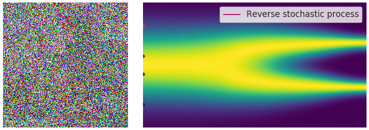
From: Yang Song's blog . The image (left) starts as random pixel values pulled from $\mathcal{N}(0,I_d)$, and is gradually denoised to a coherent image. The 2D graph (right) shows that we start at a simple symmetric distribution, and move towards something more complicated ($P_{data}$)
Conditional Generation and Classifier-Free Guidance
We now have the full setup for building a diffusion model ready! However, you'll notice that our sampling procedure has no information about the label we want to generate. In the current state, our model would just randomly pull from the learned $P_{data}$. This is called unconditional generation, and diffusion models can still generate high quality samples like this. However, it may be useful to perform conditional generation (also referred to as guided generation), where we basically give our U-Net information about labels for each sample, during training and inference. Formally, we'd say that we want to sample $x_0 \sim P_{data}(x|y)$ where $y \in \{0,1,2,...,n\}$ for $n$ classes. In practice, this is quite easy to implement, now we'd want to learn a guided score-network $s_t^{\theta}(x | y)$. To do this, we can just sample $(x_0, y) \sim P_{data}$ (i.e we'd need the sample and the label) during training. We pass label information onto $s_t^{\theta}(x | y)$ by having it inject this information (stored via some kind of embedding, like $t$) into each residual unit of our U-Net.
We can go even further with conditional generation, using a technique called Classifier-Free Guidance (CFG) [5]. Basically, CFG lets us control the guided generation's effect, which leads to significantly better samples. Also, notice the name classifier-free guidance, this is an improved version of the original (and apparently no longer used) method that lets us control the strength of guidance. Without getting too much into it, the old iteration relied on Bayes' rule, which flips the conditional probability, so one of the terms ends up needing a $p_t(y|x)$ ($y$ given $x$, not $x$ given $y$). $p_t(y|x)$ is a classifier because it is basically gives us the class probability, given a noisy sample $x$. Having to train a classifier is obviously costly, and can lead to instability. I will first present the main equation for CFG:
Here, $w > 1$ specifies the guidance strength. None of that inverted probability $(y|x)$ here, but we do have both $s_t^{\theta}(x|y)$, the conditional score network and $s_t^{\theta}(x)$, the unconditional score network. So in order to implement CFG, we'd need both the conditional and unconditional score networks, then we can just use $\tilde{s}_t^{\theta}(x|y)$ with a given $w$ as our score predictor during the reverse process. Does this mean we have to train two score networks? Nope! Thankfully, there is a way to get both during training.
The technique we use to get the unconditional and conditional scores simultaneously and in one model is actually quite simple. We add a new hyperparameter $\eta$, this is the probability that we will drop the label for a given sample during training, and have the model learn the score estimate unconditionally. The way to "drop a label" in practice consists of adding a new class to our $y$ set. We'll call it the null class, so now $y \in \{0,1,2,...,n, \varnothing\}$ where $y = \varnothing$ is the null label. That's pretty much it. Our score network $s_t^{\theta}(x|y)$, will now be trained such that if $y$ is $\varnothing$, then the generation is class-less (which means $s_t^{\theta}(x|\varnothing) = s_t^{\theta}(x)$). We now have everything we need to implement CFG, all we need to do is use $\tilde{s}_t^{\theta}(x|y)$ during generation. I'd suggest looking through my code for this, it truly is simple to implement.
Implementation Details
My experiments were performend on MNIST Digits, the dataset was divided into training and validation (so we can keep track of validation loss during training). It should be noted that MNIST Digits is extremely simple (10 classes, 28x28 images, single-channel, primitive shapes), but it does show that at least my implementation is functional. I'm yet to try my model on other datasets. CIFAR-10 might be a good one, I don't see why it wouldn't work with the appropriate adjustments in u-net size, and hyperparameters.
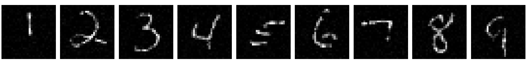
Example outputs of score-matchign diffusion trained on MNIST Digits, for classes 1-9. Trained for ~130 epochs, LR=1E-4, $\eta$=0.1, $\beta_{min}=0.1$ and $\beta_{max}=20$. Convolutional U-Net with channels [64,128,256], 2 residual units per block, time embed dim of 128.
References
-
Zeghidour, N., Luebs, A., Copet, J., Tagliasacchi, M., Grangier, D., & Aharoni, A. (2021). SoundStream: An End-to-End Neural Audio Codec. arXiv:2107.03312.
-
Song, Y. & Ermon, S. (2020). Score-Based Generative Modeling through Stochastic Differential Equations. arXiv:2011.13456.
-
Holderrieth, P. & Erives, E. (2025). An Introduction to Flow Matching and Diffusion Models. arXiv:2506.02070.
-
Ho, J., Jain, A. & Abbeel, P. (2020). Denoising Diffusion Probabilistic Models. arXiv:2006.11239.
-
Ho, J. & Salimans, T. (2022). CLASSIFIER-FREE DIFFUSION GUIDANCE. arXiv:2207.12598.